PianoID: Inverse Physical Modelling of the Piano
The Challenge
Matching a physical piano model to a real instrument is an ill-posed inverse problem. From a handful of notes recorded in an untreated room, you have to recover hundreds of coupled parameters: string stiffness and inharmonicity, frequency-dependent losses, unison detuning, nonlinear hysteretic hammer felt, and soundboard radiation. Black-box neural capture (the way amp modellers work) cannot help, because a piano has no input jack for a test sweep, and a snapshot trained on a few notes cannot extrapolate to 88 keys, 128 velocities, pedals and sympathetic resonance. End-to-end gradient descent through a recursive waveguide or FDTD scheme is not much better: backpropagating through tens of thousands of time steps is unstable, and a fraction-of-a-percent error in f₁ or B misaligns the upper partials so badly that spectral losses stop carrying useful gradients.
My Role & Collaborators
I designed and built the real-time JUCE/C++ engine (codename sora), the plugin UI and the analysis tooling, and I'm leading the calibration research.
Our Solution
The pipeline exploits the piano's physical modularity, so the parameters that can be solved in closed form never go near an optimiser. Stage 1 is analytical: a Partial Frequencies Deviation loop (Rauhala–Välimäki) jointly locks f₁ and B from f_k = k·f₁·√(1 + B·k²), restricted to partials 6–12 on double-wound bass strings. Per-partial decay rates σ_k ≈ b₁ + b₃·ω_k² come from STFT tracking with Bank's τ⁴-weighted regression, and unison detuning is read off the beat nodes. Stage 2 takes 9–15 anchor notes to all 88 keys with Rigaud's dual-bridge model, B(m) = exp(b_B(m)) + exp(b_T(m)), and rebuilds the Railsback stretch curve from octave-type matching. With the partials already aligned, Stage 3 becomes a well-conditioned search over Stulov's hysteretic felt parameters {H₀, p, τ₀, ε_h, α}: an encoder trained offline on synthetic renders of the engine gives the starting point, and Ceres (Jet autodiff, Levenberg–Marquardt) or NLopt refines it against a multi-resolution STFT loss on the first 100 ms. Stage 4 recovers the soundboard, cabinet and microphone response by Tikhonov-regularised spectral division against the simulated bridge force, then fits a minimum-phase FIR, an FDN tail and the damper and release behaviour. The target is a full calibration in under a minute on a background CPU thread, fully offline.
Key Techniques
- Stiff lossy string PDE (Chaigne–Askenfelt) realised as modal synthesis up to 12 kHz
- Joint f₁ / inharmonicity B estimation (PFD algorithm), with a double-wound bass correction
- Frequency-dependent loss fitting, σ_k ≈ b₁ + b₃·ω_k², with perceptually weighted least squares
- Sparse-to-dense compass interpolation (Rigaud dual-bridge model) and Railsback stretch tuning
- Nonlinear hysteretic hammer inverse: neural initialisation plus local Ceres / NLopt refinement
- Regularised spectral deconvolution of soundboard radiation, minimum-phase FIR, FDN reverb
- Thread-safe background calibration in JUCE with an atomic parameter swap into the audio thread
- stage inverse
- 4
- keys from ~10
- 88
- modal bandwidth
- 12 kHz
Results
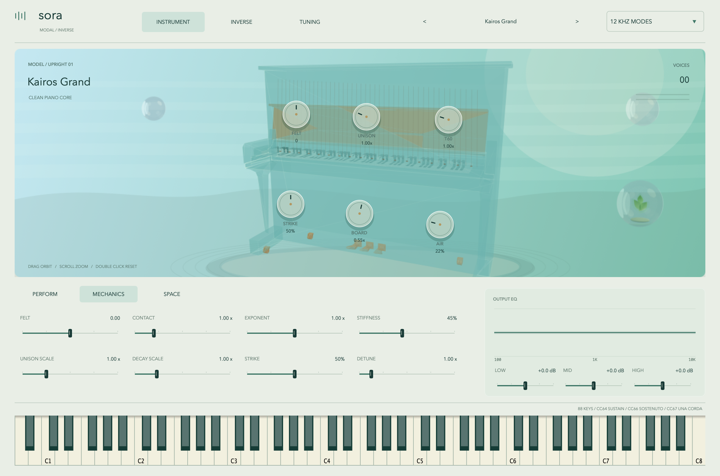
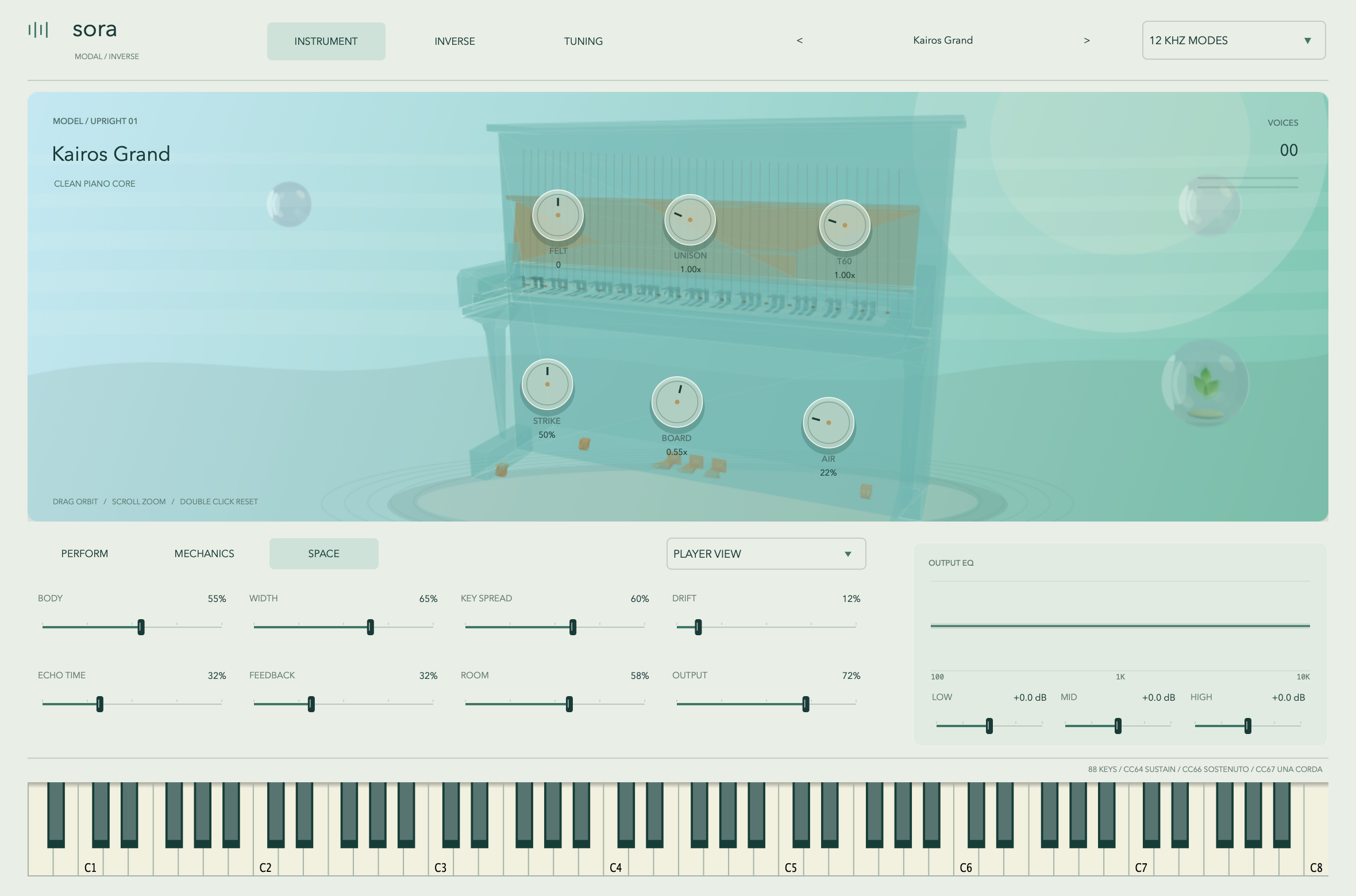
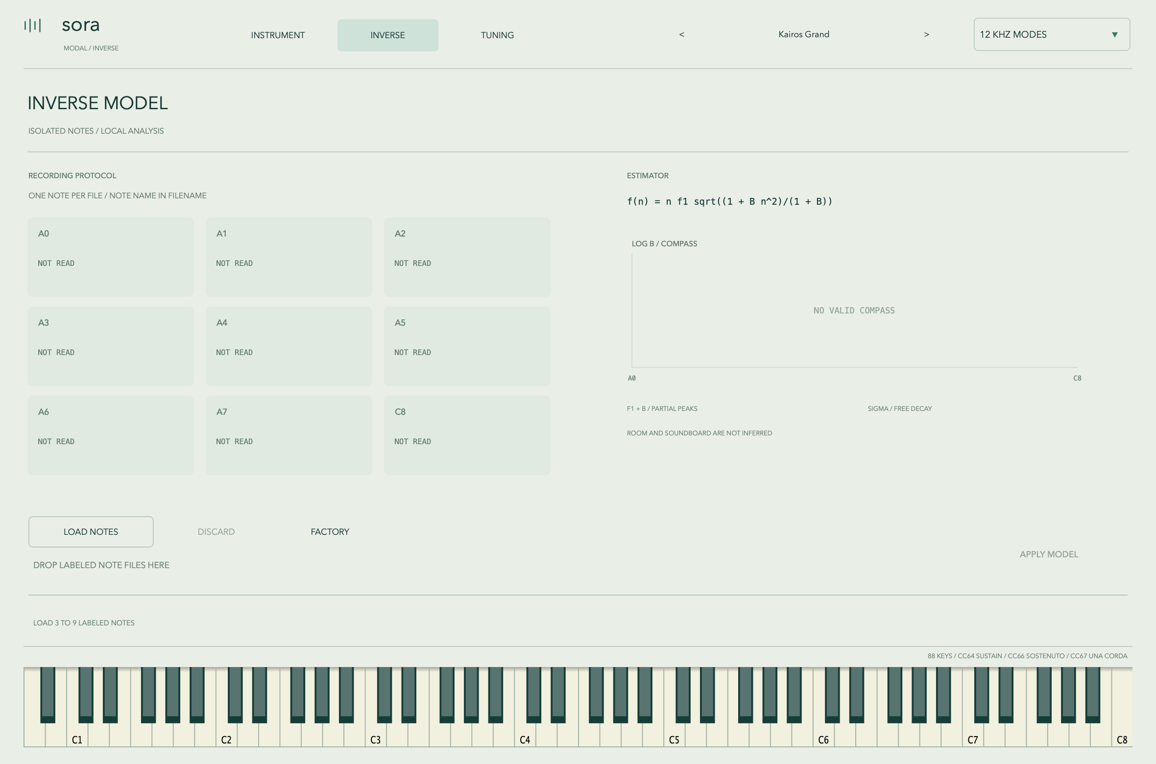
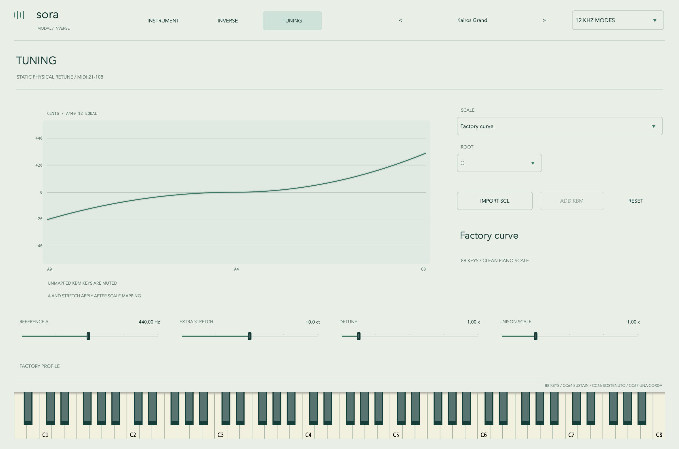
Running today in the JUCE prototype: the forward model (strings, hammer, damping, unison, pedals, soundboard and air stages), per-note f₁, B and decay estimation from 3–9 labeled notes, the log-B compass view and stretch tuning with Scala import. In progress: the full Stage 1 loss and beating extraction, the hammer inverse (Stage 3) and soundboard deconvolution (Stage 4). Open questions: identifiability of the felt parameters, model mismatch, and generalising to notes and dynamics left out of the fit.
System Architecture
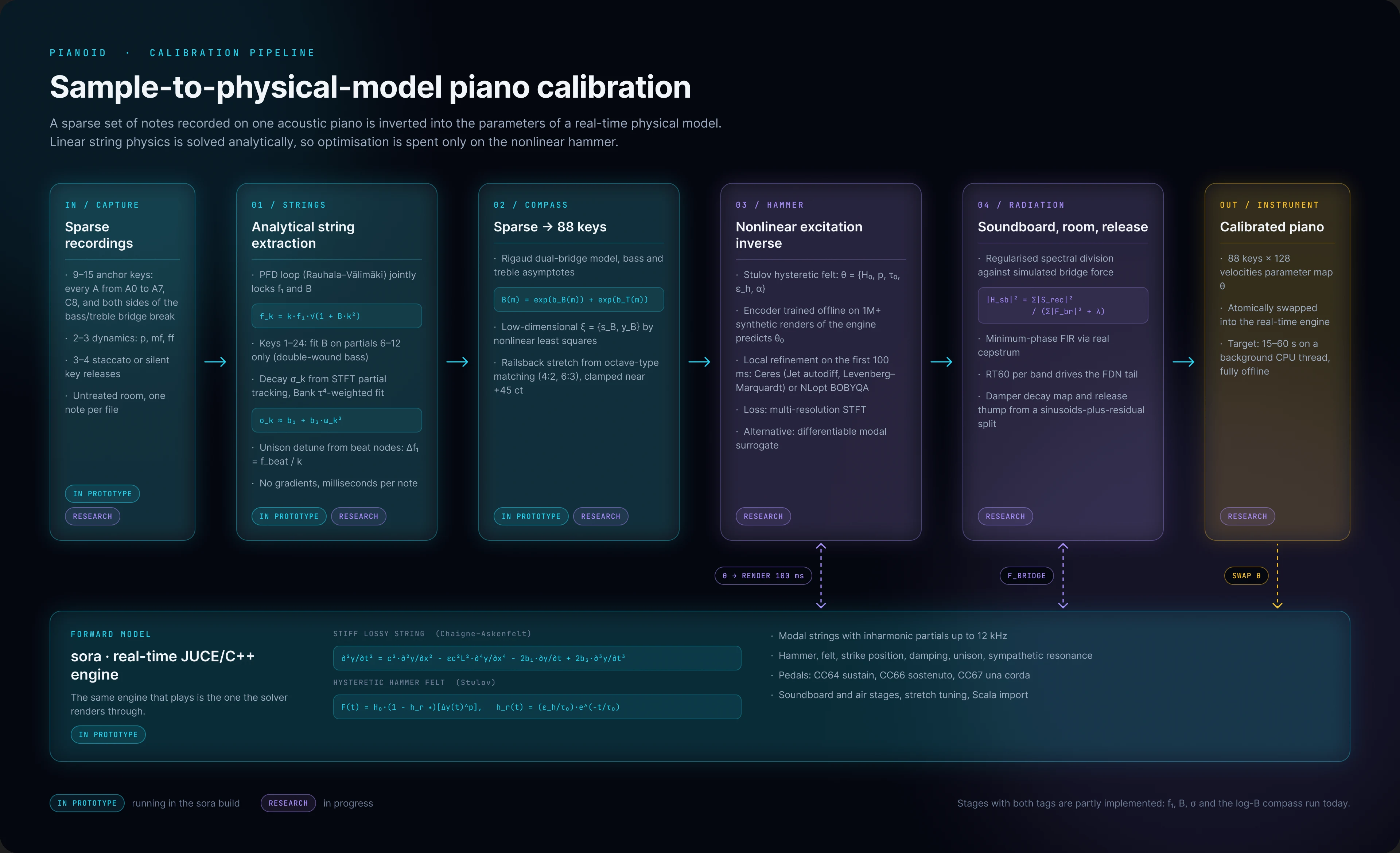
Click the diagram to open it full size.
Project Gallery